Simulations of electromagnetic waves
with python-meep
Introduction
MEEP is an open-source implementation of the finite-difference time-domain (FDTD) algorithm. It can compute the propagation of an electromagnetic wave through very complicated structures, using realistic material models (including dispersion, conductivity, anisotropy or nonlinearities), distributed computing and combination of time-domain and frequency-domain solver.
MEEP is controlled by command-line interface which requires some programming. This has a good purpose, as experienced users may employ MEEP for problems where more user-friendly simulation software does not provide enough versatility (e. g. for automated optimization of the structure, tight integration with other software packages or research in modern areas of physics). On the other hand, it may be quite disappointing to start using MEEP: Setting up a realistic simulation is usually a challenging scientific task on its own, and with MEEP one also needs to write a working code. I will try to provide the reader with a module and examples that should help to focus on the scientific part of the task.
The examples here are based on the python-meep interface. The core of MEEP is written in efficient C++ code, and that can be either directly linked into another C++ program, or an interface can be generated that allows to access the functions from high-level languages. One of the interfaces is python-meep (with its official website at Ghent university). Another interface links MEEP to the Scheme language, which is also extensively used on the official MEEP website. The reason why I chose the Python interface lies in my preference of Python syntax as well as in many excellent Python modules available (scipy, matplotlib and mayavi2 will be used in the examples here).
This page does not aim to substitute the official MEEP documentation nor Python-Meep documentation. I will simply try to provide the reader with several working examples. Get inspired and reuse them as you need! Before we get to writing the first simulation, we will discuss the installation procedure and multiprocessing.
Installing MEEP and python-meep
Notes
While it is possible to install MEEP from the debian/ubuntu repository (older version of MEEP 1.1.1 up to Ubuntu 14.04, newer version 1.2.1 on), here we will show how to compile a newer version from source. The python-meep interface has always to be compiled against the MEEP binary present in the system.
MEEP can use the MPI 2.1 protocol (Message Passing Interface) for multiprocessing. This protocol has several implementations, of which at least MPICH and OpenMPI are in the linux repositories. They seem to work the same, so for simplicity, we choose the latter and compile everything with support for MPI. If our simulation environment was built without support for multiprocessing, it would be simply called meep and imported as import meep. But as we compile with MPI support, all related names are are derived from meep-mpi, so the python module is named meep_mpi (so the command for import changes to import meep_mpi as meep).
For compilation, one has to: 1) compile new libctl for meep to work, 2) install all other dependencies, 3) compile MEEP so that the libmeep_mpi.so library is installed in the system, 4) download and build the python-meep module. All these steps are covered by the following blue box, so you may simply copy the commands to your terminal. It was tested to work flawlessly on many systems, so in case of any problems, write me an e-mail and I will try to fix it.
The following compilation procedure has been tested on Debian-based Linux distributions, but there should be no principial limitation in running meep and python-meep on and other systems, too. The same holds for older Ubuntu 10.10 and 11.04, but one has to change "guile-2.0-dev" to older "guile-1.8-dev". Hereby I thank Martin Fiers for his kind help with the installation process.
Compilation on Debian/Ubuntu
The procedure presented below enables one:
- ... to use the latest version of meep and the compiled code might also run a bit faster on the machine it was built on.
- ... to use the multiprocessing,
- ... to install on 32-bit or 64-bit architecture without any changes in the following commands,
- ... and to install meep and python-meep into the /usr/local/ directory to prevent collision with the official version of meep that may be installed from repository.
#!/bin/bash
## This is a compilation procedure that worked for me to setup the python-meep
## with some utilities on a Debian-based system.

## --- Settings ---------------------------------------------------------------

## (Optional) Install utilities
sudo apt-get update
sudo apt-get install python-matplotlib mayavi2 h5utils imagemagick -y

## --- Build dependencies -----------------------------------------------------
## (list obtained from https://launchpad.net/ubuntu/quantal/+source/meep)
sudo apt-get update
sudo apt-get install -y autotools-dev autoconf chrpath debhelper gfortran \
    g++ git guile-2.0-dev libatlas-base-dev libfftw3-dev libgsl0-dev \
    libharminv-dev libhdf5-openmpi-dev liblapack-dev pkg-config zlib1g-dev

## On Ubuntu 14.04 or older, the version of `libctl-dev' from repository is too old
wget http://ab-initio.mit.edu/libctl/libctl-3.2.1.tar.gz
tar xzf libctl* && cd libctl-3.2.1/
./configure LIBS=-lm  &&  make  &&  sudo make install
cd ..

## --- MEEP (now fresh from github!) --------------------------------------------
## Skip this line if no multiprocessing used (also install correct libhdf5-*-dev)
meep_opt="--with-mpi"; sudo apt-get -y install openmpi-bin libopenmpi-dev

export CFLAGS=" -fPIC"; export CXXFLAGS=" -fPIC"; export FFLAGS="-fPIC"
export CPPFLAGS="-I/usr/local/include"
export LD_RUN_PATH="/usr/local/lib"

## Note: If the git version was unavailable, use the failsafe alternative below
git clone https://github.com/stevengj/meep
cd meep/
./autogen.sh $meep_opt --enable-maintainer-mode --enable-shared --prefix=/usr/local  # exits with 1 ?
make  &&  sudo make install
cd ..

## Failsave alternative: download the 1.2.1 sources (somewhat obsoleted)
#wget http://jdj.mit.edu/~stevenj/meep-1.2.1.tar.gz && tar xzf meep-1.2.1.tar.gz && mv meep-1.2.1 meep
#cd meep/
#./configure $meep_opt --enable-maintainer-mode --enable-shared --prefix=/usr/local  &&  make  &&  sudo make install
#cd ..

## --- PYTHON-MEEP ------------------------------------------------------------
## Install python-meep dependencies and SWIG
sudo apt-get install swig python-dev python-numpy python-scipy -y
## Get the latest source from green block at https://launchpad.net/python-meep/1.4
wget https://launchpad.net/python-meep/1.4/1.4/+download/python-meep-1.4.2.tar
tar xf python-meep-1.4.2.tar  &&  cd python-meep/

## If libmeep*.so was installed to /usr/local/lib, this scipt has to edit the installation scripts (aside
## from passing the "-I" and "-L" parameters to the build script).
pm_opt=`echo $meep_opt | sed 's/--with//g'`
sed -i -e 's:/usr/lib:/usr/local/lib:g' -e 's:/usr/include:/usr/local/include:g' ./setup${pm_opt}.py
sed -i -e '/custom.hpp/ a export LD_RUN_PATH=\/usr\/local\/lib' make${pm_opt}
sed -i -e 's/#global/global/g' -e 's/#DISABLE/DISABLE/g' -e 's/\t/    /g'  meep-site-init.py
sudo ./make${pm_opt} -I/usr/local/include -L/usr/local/lib
More information on running parallel meep is documented on the meep wiki.
Installing MEEP 1.2.1 from repository on Ubuntu 14.10
In Ubuntu 14.10 and probably also its newer versions, MEEP 1.2.1 with all its dependencies is available in the repository.
Python-meep needs however to be still built, and I added a little fix to its building script that had to be done in Ubuntu 14.10. (I tested this for the MPI-enabled version only, but it should work with the non-mpi one, too.)
Note that in the packaged version 1.2.1, the frequency domain solver (function solve_cw()) is probably broken. As of 2015, if frequency-domain solver is to be used, one has to compile the latest version from source (see above).
#!/bin/bash
apt-get install swig python-dev python-numpy python-scipy -y

## --- MEEP (from the Ubuntu repository) ----------------------------------------
apt-get install meep-openmpi libmeep-openmpi-dev

## --- python-meep -------------------------------------------------
wget https://launchpad.net/python-meep/1.4/1.4/+download/python-meep-1.4.2.tar
tar xf python-meep-1.4.2.tar  &&  cd python-meep/
sed -i -e 's/#global/global/g' -e 's/#DISABLE/DISABLE/g' -e 's/\t/ /g'  meep-site-init.py
sed -i -e '/libraries =/s/meep_mpi/meep_openmpi/g' setup-mpi.py  	# (a little fix)
sudo ./make-mpi
C importompilation procedure for MEEP 1.2.1 and python-meep on Mac OS-X
A guide for Mac OS-X Yosemite is in the mail archive (February 2015)
Performance and multiprocessing
The FDTD time-stepping algorithm is typical by performing relatively simple arithmetics on big data arrays. For typical simulations, tens to hundreds of megabytes in memory are updated each step. On many computers, the bottleneck limiting the speed of computation is not the CPU frequency, but the frequency of the RAM or even more likely, the front side bus data throughput [see also].
The speed of computation depends on many parameters and paralellisation may or may not be advantageous. For example, I tested MEEP on three different computers:
- Notebook Asus F9E with Core2 Duo performs better when running single process than two processes, due to some overhead of multiprocessing. It is therefore fastest to get along with the non-MPI version of meep here, although the second processor core remains idle.
- On my desktop computer with 3 GHz dual-core Intel i3 processor and dual-channel RAM, multiprocessing brings some speed advantage, although it is by far below 200 %. In some cases, the bottleneck can be in the front-side bus instead of the CPU core. Launching more than 2 processes always gave me even worse results. (A related question by Giovanni.).
- Finally, on a HP Z820 workstation with 2x4 Intel Xeon E5-2643 cores and 64 GB RAM, the CPU-RAM communication is evidently fast enough and running simulation in 8 processes reduces computational time roughly five times, as is illustrated in the following figure:

Logarithmic plot of time needed for one time step, depending on the simulation volume and processor cores used for the computation. Comparison of the Z820 workstation denoted as Lorentz and my notebook.
From comparison of the measured speed with linear extrapolation, one sees that the computing power scales well with processor cores employed (except for very small problems).
To conclude, the answer depends on your computational setup: for older dual-core computer probably not, for a new multiprocessor computer definitely yes -- one has to try it out in practice.
Simulation basics
Conventions
In order to simplify the interpretation of results, all the simulations on this page will use the SI units (e. g. meters, seconds, volts...). In the MEEP's routines, the speed of light is defined as 1.0 (instead of 2.997e8 m/s), and also the vacuum impedance is 1.0 (instead of 377 Ohm). Therefore, when we feed MEEP with some frequency, we always divide it by c=2.997e8 and when MEEP returns some frequency value to us, we in turn multiply it by c. Opposite procedure has to be done when handling time units etc. As long as linear systems are simulated, this convention makes no qualitative difference in the results; see also Meep unit Wiki.)
We assume the reader will probably make use of the multiprocessing version, so all examples presented here are MPI-enabled. This means that they use
import meep_mpi as meepand that all file outputs are carefully tested to work even when 16 threads are running in parallel. If you wish to use the non-MPI version, just remove the "_mpi" from the module name and import meep simply as:
import meep
We also always keep all MEEP's functions in their original namespace, which makes the code easier to read and reuse. (This means we will use "import meep_mpi as meep" instead of "from meep_mpi import *".)
Minimal simulation of dielectric sphere
Let us look at a 25 lines of python code that already produce an interesting output. You may either launch an interactive python session and insert the commands one by one, or copy all the code into one python file, or download the file here: minimal.py.
Imports
First, we import meep_mpi and define some constants. The real dimensions of the simulated volume will be 2x2x5 micrometers with a reasonable voxel size of 50 nm. (Therefore we will later compute in 40x40x100=160000 voxels.)
#!/usr/bin/env python
import meep_mpi as meep
x, y, z, voxelsize = 2e-6, 2e-6, 5e-6, 50e-9
Python-meep is based on the object model, so first we create an object defining the volume where all simulation is run.
vol = meep.vol3d(x, y, z, 1/voxelsize)
Now we define a tiny transparent dielectric sphere, with relative permittivity 10 and diameter 600 nm, in the center of volume.
The following code may look a little tricky, because of using the callback. The C++ code of MEEP now requires us to provide it a function, named double_vec(), that accepts the position and returns the value of permittivity. It is quite unusual to call python from C++, but it is possible and MEEP uses it as an option to load permittivity, susceptibilities or field vectors. (For technical reasons it requires that double_vec() is a method of an object that inherits from meep.Callback. Before the object pointer is passed to the C++ core of MEEP, its method __disown__() must be called once.)
After we tell MEEP what callback to use, we may create the structure object. Repeated calling the double_vec() function takes few seconds. After that, the struct object stores the value of permittivity in each voxel.
class Model(meep.Callback):
    def double_vec(self, r):
        if (r.x()-1e-6)**2+(r.y()-1e-6)**2+(r.z()-2.5e-6)**2 < .6e-6**2:
            return 10
        else:
            return 1

model = Model()
meep.set_EPS_Callback(model.__disown__())
struct = meep.structure(vol, meep.EPS)
Finally, we also create the fields object and give it one source, that will excite the Ex and Hy field components with an ultrashort optical pulse, with center frequency of 300 THz and spectral width of 500 THz. By default, the volume boundaries behave as perfect conductor. The source looks like a current sheet covering one plane of the simulation volume, that is, all points where z=.1e-6 m.
f = meep.fields(struct)
f.add_volume_source(meep.Ex,
        meep.gaussian_src_time(300e12/3e8, 500e12/3e8),    # (setting frequency = dividing by speed of light)
        meep.volume(meep.vec(0,0,.1e-6), meep.vec(2e-6,2e-6,.1e-6)))
Everything is prepared! We may now let the source transmit a wave and let it propagate through the structure for, say, 30 femtoseconds. The computational time will be a bit longer (roughly 20 s). MEEP writes out the progress each 4 seconds.
while f.time()/3e8 < 30e-15:   # (retrieving time = dividing by speed of light)
    f.step()
We are now free to access any field component at any point in the space. Note the fields are complex-valued.
print f.get_field(meep.Ex, meep.vec(.5e-6, .5e-6, 3e-6))
Much better insight is provided by 3D visualisation. Let us export the real part of Ex field component:
output = meep.prepareHDF5File("Ex.h5")
f.output_hdf5(meep.Ex, vol.surroundings(), output)
del(output)
The Ex.h5 file can be converted into VTK format. If you have h5utils installed, run in bash or your favourite shell:
h5tovtk Ex.h5Now launch mayavi2, open the resulting
Ex.vtk file, add a ScalarCutPlane or IsoSurface objects and view the field amplitude in 3D. You may experiment changing the structure or letting the simulation timestepping continue to a later time and load the new field into mayavi2 to compare how it evolves. But if you wish to run some realistic simulation, do not base your code on this simplistic example. The more elaborate examples below may save you a lot of coding.

Screenshot from mayavi2 with a ScalarCutPlane module, showing the x-component of electric field. From right to left we see the wave that propagated around the sphere, then a wave that still propagates in the denser medium of the sphere (being focused at rear interface) and at the left there is also a weak reflected wave.
A more elaborate simulation with meep_utils.py and meep_materials.py
Please download meep_utils.py and meep_materials.py to the working directory. You may of course use these commands in bash:
wget http://fzu.cz/~dominecf/meep/scripts/meep_utils.py
wget http://fzu.cz/~dominecf/meep/scripts/meep_materials.py
The first module contains convenience functions that spare a lot of non-scientific programming, while the second is an easily extensible library of MEEP materials. In the following we will make use of them to run a practical simulation. You may download the simulation script, but it may be more instructive to separate it into logical parts.
Initialisation and imports
Similar as before, we import the common moduli (time, sys, os), the scientific ones (numpy, meep) and the two we just downloaded above (meep_utils, meep_materials). The last import line is again for those without multiprocessing.
#!/usr/bin/env python
#-*- coding: utf-8 -*-
""" run_sim.py - an example python-meep simulation of a dielectric sphere scattering a broadband impulse,
illustrating the use of the convenient functions provided by meep_utils.py
(c) 2014 Filip Dominec, see http://fzu.cz/~dominecf/meep/ for more information """

import numpy as np
import time, sys, os
import meep_utils, meep_materials
from meep_utils import in_sphere, in_xcyl, in_ycyl, in_zcyl, in_xslab, in_yslab, in_zslab, in_ellipsoid
import meep_mpi as meep
#import meep
c = 2.997e8

sim_param, model_param = meep_utils.process_param(sys.argv[1:])
Defining the model
Similarly to the simplest simulation presented above, we create a class that defines the structure. It accepts some relevant named parameters with reasonable default values. Other properties of the model are constants defined in the body of the __init__ function. Some of them should always be defined, as they are used by the simulation script.
The list self.materials stores all materials used. The constructor of each material is pointed to some function that defines where the material is -- it must return self.return value in the material, and 0 otherwise. But the condition defining the material shape is absolutely arbitrary; it can be some implicit function, it can be composed of many logical operations with primitives (sphere, cylinder, slab), it can be complicated and procedurally generated. With one limitation: the materials should never overlap (except for when you know what you do).
Note this class inherits from meep_utils.AbstractMeepModel the capability to define multiple materials with one class. (Moreover, each material can come with possibly multiple properties such as polarizabilities, conductivity, nonlinearity etc.) The technical details are not important; you may look at meep_utils.py for the trick.
class SphereWire_model(meep_utils.AbstractMeepModel): #{{{
    def __init__(self, comment="", simtime=10e-12, resolution=6e-6, cells=1, monzc=0e-6, padding=50e-6,
            radius=25e-6, spacing=75e-6, wlth=10e-6, wtth=10e-6, Kx=0, Ky=0, dist=25e-6):
        meep_utils.AbstractMeepModel.__init__(self)        ## Base class initialisation
        self.simulation_name = "SphereWire"
        monzd=spacing

        self.register_locals(locals())          ## Remember the parameters

        ## Constants for the simulation
        self.pml_thickness = 20e-6
        self.monitor_z1, self.monitor_z2 = (-(monzd*cells)/2+monzc-padding, (monzd*cells)/2+monzc+padding)
        self.simtime = simtime      # [s]
        self.srcFreq, self.srcWidth = 1000e9, 2000e9     # [Hz] (note: gaussian source ends at t=10/srcWidth)
        self.interesting_frequencies = (0e9, 2000e9)     # Which frequencies will be saved to disk

        self.size_x = spacing
        self.size_y = spacing
        self.size_z = 60e-6 + cells*monzd + 2*self.pml_thickness + 2*self.padding

        ## Define materials
        self.materials = [meep_materials.material_TiO2_THz(where = self.where_TiO2)]
        if not 'NoMetal' in comment:
            self.materials += [meep_materials.material_Metal_THz(where = self.where_metal) ]
        self.TestMaterials()

        f_c = 2.997e8 / np.pi/self.resolution/meep_utils.meep.use_Courant()
        meep_utils.plot_eps(self.materials, mark_freq=[f_c])

    # each material has one callback, used by all its polarizabilities (thus materials should never overlap)
    def where_metal(self, r):
        if (in_yslab(r, cy=0e-6, d=self.wtth)) and in_zslab(r, cz=0, d=self.wlth):
            return self.return_value            # (do not change this line)
        return 0

    def where_TiO2(self, r):
        if (in_sphere(r, cx=0, cy=-self.size_x/2, cz=0, rad=self.radius) or
                in_sphere(r, cx=0, cy=self.size_x/2, cz=0, rad=self.radius)):
            return self.return_value             # (do not change this line)
        return 0
#}}}
Initializing the instances model, volume and structure
# Model selection
model = SphereWire_model(**model_param)
if sim_param['frequency_domain']: model.simulation_name += ("_frequency=%.4e" % sim_param['frequency'])

## Initialize volume and structure according to the model
vol = meep.vol3d(model.size_x, model.size_y, model.size_z, 1./model.resolution)
vol.center_origin()
s = meep_utils.init_structure(model=model, volume=vol, sim_param=sim_param, pml_axes=meep.Z)
Defining fields
## Create fields with Bloch-periodic boundaries (any transversal component of k-vector
## is allowed, but may not radiate)
f = meep.fields(s)
f.use_bloch(meep.X, -model.Kx/(2*np.pi))
f.use_bloch(meep.Y, -model.Ky/(2*np.pi))
Defining wave source
## Add a source of the plane wave (see meep_utils for definition of arbitrary source shape)
if not sim_param['frequency_domain']:           ## Select the source dependence on time
    #src_time_type = meep.band_src_time(model.srcFreq/c, model.srcWidth/c, model.simtime*c/1.1)
    src_time_type = meep.gaussian_src_time(model.srcFreq/c, model.srcWidth/c)
else:
    src_time_type = meep.continuous_src_time(sim_param['frequency']/c)
srcvolume = meep.volume(
        meep.vec(-model.size_x/2, -model.size_y/2, -model.size_z/2+model.pml_thickness),
        meep.vec( model.size_x/2,  model.size_y/2, -model.size_z/2+model.pml_thickness))
f.add_volume_source(meep.Ex, src_time_type, srcvolume)
Defining outputs
## Define monitors planes and visualisation output
monitor_options = {'size_x':model.size_x, 'size_y':model.size_y, 'Kx':model.Kx, 'Ky':model.Ky}
monitor1_Ex = meep_utils.AmplitudeMonitorPlane(comp=meep.Ex, z_position=model.monitor_z1, **monitor_options)
monitor1_Hy = meep_utils.AmplitudeMonitorPlane(comp=meep.Hy, z_position=model.monitor_z1, **monitor_options)
monitor2_Ex = meep_utils.AmplitudeMonitorPlane(comp=meep.Ex, z_position=model.monitor_z2, **monitor_options)
monitor2_Hy = meep_utils.AmplitudeMonitorPlane(comp=meep.Hy, z_position=model.monitor_z2, **monitor_options)

slice_makers =  [meep_utils.Slice(model=model, field=f,
		components=(meep.Dielectric), at_t=0, name='EPS')]
slice_makers += [meep_utils.Slice(model=model, field=f,
		components=meep.Ex, at_x=0, min_timestep=.05e-12, outputgif=True)]
slice_makers += [meep_utils.Slice(model=model, field=f,
		components=meep.Ex, at_t=2.5e-12)]
Running the simulation!
if not sim_param['frequency_domain']:       ## time-domain computation
    f.step()
    dt = (f.time()/c)
    meep_utils.lorentzian_unstable_check_new(model, dt)
    timer = meep_utils.Timer(simtime=model.simtime); meep.quiet(True) # use custom progress messages
    while (f.time()/c < model.simtime):                               # timestepping cycle
        f.step()
        timer.print_progress(f.time()/c)
        for monitor in (monitor1_Ex, monitor1_Hy, monitor2_Ex, monitor2_Hy): monitor.record(field=f)
        for slice_maker in slice_makers: slice_maker.poll(f.time()/c)
    for slice_maker in slice_makers: slice_maker.finalize()
    meep_utils.notify(model.simulation_name, run_time=timer.get_time())
else:                                       ## frequency-domain computation
    f.step()
    f.solve_cw(sim_param['MaxTol'], sim_param['MaxIter'], sim_param['BiCGStab'])
    for monitor in (monitor1_Ex, monitor1_Hy, monitor2_Ex, monitor2_Hy): monitor.record(field=f)
    for slice_maker in slice_makers: slice_maker.finalize()
    meep_utils.notify(model.simulation_name)
Processing the reflection and transmission
This is an absolutely optional step, applicable only to simulations where the recording planes make sense.
## Get the reflection and transmission of the structure
if meep.my_rank() == 0:
    freq, s11, s12 = meep_utils.get_s_parameters(monitor1_Ex, monitor1_Hy, monitor2_Ex, monitor2_Hy,
            frequency_domain=sim_param['frequency_domain'], frequency=sim_param['frequency'],
            maxf=model.srcFreq+model.srcWidth, pad_zeros=1.0, Kx=model.Kx, Ky=model.Ky)
    meep_utils.savetxt(freq=freq, s11=s11, s12=s12, model=model)
    #import effparam        # process effective parameters for metamaterials
Finalizing
As the absolutely last command, we must include meep.all_wait. Otherwise the first process that succesfully terminates causes premature termination of all other. This often manifests as a corrupt or incomplete HDF5 file being saved.
It may save some work to write down which directory came the most recent simulation.
with open("./last_simulation_name.txt", "w") as outfile: outfile.write(model.simulation_name)
meep.all_wait()         # Wait until all file operations are finished
That's all. The multiprocessing simulation always ends with a warning mpirun has exited ... without calling "finalize", but this is harmless.
mpirun -np 4 python run_sim.py
Overview of the meep_utils.py module
The previous example may serve as a good basis for the simplest simulations. The structure it uses is built of nondispersive materials and the resulting fields can be viewed in Mayavi2 or processed by the MEEP's builtin postprocessing functions. However, when one decides to compute some practical problems, usually a lot of pre- or postprocessing code has to be written. Programming in python provides great possibilities, but the most often needed functions are in fact quite basic. In order to prevent the user from having to reinvent the same code over and over, we present the meep_utils.py module in the next paragraphs.
This is not an exhaustive documentation, but rather an "advertisement" for the functions available. Their exact usage will be illustrated in the next chapter, where one more elaborated simulation employing all the following functions is presented.
Definition of the structure
In the simple simulation above, we were already forced (by technical reasons) to use an object to define the permittivity. We can fully take advantage of the object programming and store the whole structure in one class. This results in cleaner code and also in much easier switching between different structures to be simulated.
class AbstractMeepModel(meep.Callback)
Most of the methods defined by AbstractMeepModel simplify the (otherwise quite intimidating) interaction with python-meep's internals.
There are several ways how to define the structure in Python-meep. Unfortunately, the most convenient predefined primitives available in scheme-meep are not available in python-meep (because they are provided by libctl, which is not processed by SWIG yet).
Instead, we suggest to use the slow, but convenient callback approach: when defining the structure, MEEP calls some user-defined method for each point and each material in order to find out whether the material is or is not at the given point. Therefore it is convenient to use the following functions:
in_xslab(r,cx,d):
in_yslab(r,cy,d):
in_zslab(r,cz,d):
in_xcyl(r,cy,cz,rad):
in_ycyl(r,cx,cz,rad):
in_zcyl(r,cx,cy,rad):
in_sphere(r,cx,cy,cz,rad):
in_ellipsoid(r,cx,cy,cz,rad):
Along with the boolean operators in Python (and, or, not), they allow to construct the simulated structure in fully parametric way. Of course that one can complement them with own code, for instance to define some implicit plane like a parabolic mirror. With a little practice, one can write the structure definition quite effectively. It is very helpful to check the resulting structure in Mayavi2, as discussed below.
Dispersive materials
In many FDTD programs including MEEP, the dielectric function is defined as a sum of zero, one or more Lorentzian oscillators with a constant term. This allows one to define the losses, dispersive dielectrics, metals, etc. as needed. A separate chapter is dedicated to this topic.
Another good feature of MEEP is the frequency-domain solver. But, unfortunately, it can not handle the dispersive materials. (There is no principial problem, it only has not been implemented yet into the MEEP core, as of 2013.) To use the frequency-domain solver, one has to provide the permittivity and conductivity at the frequency of interest. The AbstractMeepModel class makes use of the following functions and classes to do everything for the user automatically.
def permittivity2conductivity()
def analytic_eps(mat, freq):
    complex_eps = mat.eps
    for polariz in mat.pol:
	complex_eps += polariz['sigma'] * polariz['omega']**2 / \\
		(polariz['omega']**2 - freq**2 - 1j*freq*polariz['gamma'])
    return complex_eps # + sum(0)
class MyHiFreqPermittivity(meep.Callback)
class MyConductivity(meep.Callback)
Using the AbstractMeepModel approach, one can now switch between time- and frequency-domain computation without any changes in the structure. The typical usage is that one may define any structure containing dispersive materials, run a standard time-domain simulation to obtain the full spectra, identify the resonance frequences and finally rerun the simulation in frequency-domain mode to see the resonant modes. Again, this will be illustrated in the next chapter.
Field output
Although MEEP defines the function that outputs one field component to a HDF5 file, it is definitely more convenient to make use of the two following classes:
class SnapshotMaker():
    """
    Saves the field vectors to a HDF5/VTK file at a given time.
    """

class SliceMaker():
    """
    Saves the field vectors from a slice to a HDF5 file during the simulation. The slice may be specified either
    by two-dimensional meep.volume() object, or by a normal ("x", "y" or "z") and the slice position on this normal.

    After simulation ends, the data are exported as GIF animation and 3D VTK file.
    Optionally, you may disable these output formats and/or enable output to many many PNG files or to a 3D HDF file.

    This function unfortunately requires command-line tools from Linux system.
    """
The SnapshotMaker class requires only two lines in the code and provides the user with the full vector output of the fields, along with the scalar output of the structure permittivity; both files are ready to be directly loaded into Mayavi2 3-D visualiser. The SliceMaker class finally outputs an animated GIF image of the field evolution in time.
If needed, any additional command-line operation can be invoked using the run_bash function.
def run_bash(cmd, anyprocess=False)
User interaction
During the time-domain simulation, the
class Timer()estimates how long the computation will take and prints out the percentage of progress (if possible).
Especially for long simulations, one usually switches to another window/desktop and continues to work. The following function makes use of the libnotify and prints a bubble when the simulation ends.
def notify()
s-parameters retrieval and processing
The following functions are somewhat application-specific: they are designed to provide the s-parameters (i. e. complex reflection and transmission) of the structure. This may be interesting particularly for the research of metamaterials, as the s-parameters can be processed to obtain the effective index of refraction of the metamaterial.
An example of reflection and transmission computation is presented both on the meep and python-meep websites. Alas, the MEEP's internal function used for recording of the fields gives the intensity only. When two
class AmplitudeMonitorPlane()objects are used to record the field, they instead retain the full information about the complex field amplitude. This is not only a requirement for the retrieval of effective parameters [Smith2002], but also an effective way to separate the forward and backward propagating waves when both E and H are recorded. Thanks to this, there is no need to run the simulation twice (with and without the structure) as is presented on the meep website.
The separation of forward and backward waves in performed by the following function:
	def get_s_parameters()
		""" Returns the frequency, s11 (reflection) and s12 (transmission) in frequency domain """
		## Separate forward and backward waves in time domain                   +-----------------+
		## (both electric and magnetic field needed for this)         -- a1 ->|MP1|--+---s12--->|MP2| -- b2 -->
		##      a ... inputs; b ... outputs                                   |MP1| s11         |MP2|
		##      1 ... front port, 2 ... rear port (on z-axis)         <- b1 --|MP1|<-`          |MP2| <- a2=0 --
		## MP1 and MP2 are monitor planes provided                              +------structure--+
and finally the
def savetxt_for_PKGraph()exports the data to an ASCII file, along with all parameters in its header.
Defining materials
The electromagnetic properties of materials depend more or less on frequency. For a time-domain calculation, they may not be loaded as an arbitrary function of frequency, but instead they have to be expressed as a sum of Lorentz resonances. This approach requires to supply only several numbers to MEEP, but it enables one to define realistic materials, such as dispersive=lossy dielectrics and metals.
In this text, we will focus on setting the permittivity only. (The permeability may be set in similar manner as permittivity. On the other hand, the electric conductivity does not have to be set for MEEP's time-domain simulation, as the complex permittivity determines it.) A lot of theoretical literature on dielectrics is available elsewhere and it is not constructive to repeat it here. Therefore we will briefly show an example of a dielectric, discuss the specifics of the metals and then we will describe how to define them in MEEP.
Lorentz model for dielectrics
The permittivity curve of some simplified dielectric may look like this:

Real (solid) and imaginary (dashed) part of permittivity for a typical dielectric
(Note that there are big differences between the quantities being plot, so we had to use the "symlog" graph which has linear scale around zero and logarithmic scales both for larger positive and negative values)
All required dielectric properties for this model are these 10 numbers:
| Description | omega | gamma | oscillator strength (sigma) |
|---|---|---|---|
| Debye relaxation around 1 GHz | 10 GHz | 100 GHz | 100 |
| Lattice vibrations | 10 THz | 1 THz | 10 |
| Electronic resonance | 500 THz | 200 THz | 1 |
| High-frequency permittivity | 1 | ||
Summary of the dielectric properties plot above
At the right corner for ultraviolet frequency around 1016 Hz, we can see that the nondispersive part of permittivity was set to 1.0. It is legal to set it to any positive real number.
- The rightmost Lorentzian resonance has frequency omega=500 THz (orange visible light) and width 200 THz. The Kramers-Kronig relations require high losses in this region, so the material would probably appear black with bluish lustre. The strength of the oscillator was set such that it adds 1.0 in the low-frequency limit. Resonances in optical region are related to the electron shell.
- The middle Lorentzian resonance is located at 10 THz and has width of 1 THz. Resonances in far infrared range are usually caused by polar lattice vibrations and present a major contribution to the low-frequency permittivity. Note that it introduces a region of negative permittivity between 10--25 THz, which is perfectly legal (unless we break the numerical stability discussed below).
- The leftmost resonance occurs around 1 GHz and it is characteristic by being overdamped, thus it is more correct to denote it as Debye relaxation. This occurs often in dielectrics and liquids when the polar molecules orient slowly along the electric field and their inertia is much smaller than friction.
(Technically, the Debye relaxation in MEEP can be defined as a Lorentz resonance, but gamma has to be at least ten times higher than omega. The relaxation will be centered around frequency given as omega**2/gamma. So when we wanted to define Debye relaxation on 1 GHz here, we set omega=10 GHz and gamma=100 GHz. Note that the spectral width of Debye relaxation cannot be set, it is given by underlying mathematics. If needed, the Cole-Cole model can be imitated by summing Debye relaxations.)
Drude model for metals
In MEEP, it is also possible to define a realistic model of metals and similar conductive materials, such as highly doped semiconductors or plasma. Again, care has to be taken on simulation stability.
Understanding the optical properties of metals may be a bit hard due to several different models being used in the literature:
1) PEC or Perfect Electric Conductor - the metal is regarded to as a medium where the electrical field is always zero. Any impinging wave is immediately screened by movement of surface charges that are supposed to have no losses and no mass. This behaviour corresponds to infinite permittivity, so it could not be plot on the graph. The walls of the MEEP's simulation volume are PEC by default, but there is probably no way to use it in python-meep so far (?). In many cases PEC is a sufficient approximation for nonresonant bulk metallic structures.
2) Lossless Drude model - the charges in metal have nonzero mass. Above a so called plasma frequency (related to their mass and concentration), the charges are not fast enough to compensate the electric field anymore and the wave starts to propagate through the metal. In such regime, the permittivity is between 0 and 1 and the material is dispersive. Well below the plasma frequency, the metal behaves similarly as PEC except for permittivity being a finite complex function diverging at low frequencies. No losses are introduced anywhere: either an impinging wave creates an exponentially decaying field just under the metal surface and all energy is reflected, or it propagates through the metal.
3) Lossy Drude model - in addition to the nonzero charge mass, it is possible to assume a finite scattering time of moving charges. This model takes into account also the finite low-frequency conductivity of metals.
4) Lossy Drude-Lorentz model - takes into account also the interband transitions, which are responsible for colour tint of some metals (copper, gold). This model is obviously important for precise simulations near optical range.

Comparison of Lossless Drude, Lossy Drude and Drude-Lorentz models for gold from microwave to UV frequencies
Technically, the Drude component may be fed to MEEP as a Lorentz resonance at an extremely low frequency, which we may denote as omega0. The strength of the oscillator then has to be set to omega_p**2/omega_0**2 (which may be a really huge number). (Another option is to try the Drude polarizability implemented in MEEP 1.2.1).
Note that in the logarithmic plot, the curves for lossy Drude[-Lorentz] model bend at the scattering frequency gamma. Below gamma, the bulk metal behaves as resistive medium, above gamma it behaves rather as inductive medium. In both cases, the metals are highly reflective. (Let us note it is still possible to make an inductor from a metal wire operating below the scattering frequency thanks to the magnetic field that can circulate around the wire. It is however not possible to make a metallic resistor that would not behave as inductor above its scattering frequency!)
The scattering frequency lies between 3--30 THz in usual metals [see comparison here].
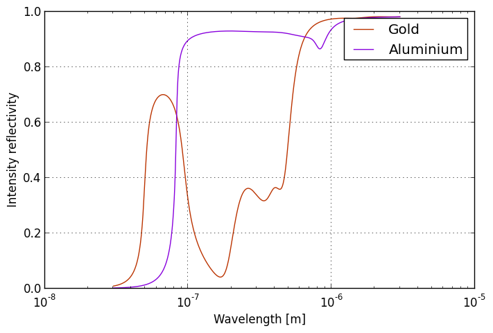
Short verification of the presented Drude-Lorentz model for gold
The Lorentz-Drude model for gold was copied as few numbers from Aaron Webster's document about metals in MEEP (see below). How is it reliable?
It is possible to verify this model by calculating optical reflectivity, and by comparing it with some experimental data. It generally proves that the values are quite precise in optical range, but may be wrong in UV.
Taking permittivity at some reasonably low frequency from the lossy Drude model, we can compute the low-frequency conductivity. Here we take (22000+3·106i) at the left border of the graph, divide by imaginary unit, multiply by the frequency (1011 Hz), by vacuum permittivity and by 2*π, obtaining 1.5·107 S/m. This is about one third of DC conductivity of gold [w]. The conductivity may be also influenced by electron mobility being dependent on frequency and by thickness of the metallic film [Johnson1972], so this is quite a good result.
Stability of simulation
So far we only discussed the theory, which is probably well known to most readers anyway. What are the requirements for the simulation to be numerically stable?
For each simulation, it is important to calculate the critical frequency = 1/π/dt = 1/π/(dx·C/c), where dx is the resolution and c is the speed of light. The Courant factor C = 0.5 for a default 3D simulation. So for example, at resolution dx = 50 nm, we get the critical frequency in UV region: 1/3.14/(5e-8*.5/3e8) = 3.82e15 Hz.
Based on some experimenting with MEEP, it can be observed that following three conditions are needed for stability of the simulation:
- At the critical frequency and above, the permittivity must be positive.
- No Lorentzian oscillator may be defined above critical frequency, and preferably not above ¾ of it to be safe.
- (Make sure your geometry provides enough space between any resonator and perfectly matched layers.)
The first and second conditions are usually fairly easy to fulfill when no metals are used. It is also easy to prevent instabilities for simulations in near-infrared or optical range, as we need a high resolution anyway. Then the critical frequency lies somewhere in the far UV region where all materials have permittivity near one.
Let us assume a typical problematic case, when we wish to compute the behavior of metallic structures in microwave or far-infrared region. The structure will have at least the size of a free-space wavelength, so it is not feasible to use the nanometric resolution here. We may, however, modify the Lossy Drude model for the metal so that the simulation will be stable with adequately low resolution.
The trick to avoid breaking the first condition consists in defining a huge non-dispersive permittivity such that it forces overall permittivity to be positive at the cricital frequency. Then the plasma frequency is the last degree of freedom remaining and we may misuse it to set the low-frequency conductivity. The mathematics can be found in the meep_materials.py file in the files section. Let us plot the permittivity graphs:

Illustration of the original Drude-Lorentz model for gold (red curve), which is unstable if too coarse timestepping is used. The improved model of metal for simulations with critical frequency at 1 THz (blue) and the same model for even lower critical frequency at 10 GHz (violet) are stable, but still maintain the low-frequency conductivity.
Material library
There is no official material library for MEEP. We can however recommend the reader to look at the permittivity spectra library at this website, which provides dielectric models for most used materials.
It is usually not too hard to search the publications for the necessary data for other materials. The most common experimental quantities are index of refraction n, index of absorption k, attenuation coefficient α = Some of the available sources of material properties are listed:
| Link | Materials covered | Format | Data columns | Note |
|---|---|---|---|---|
| A. Webster's Notes on Metals in MEEP, adapted from [Rakic1998] | metals (Ag, Al, Au, Be, Cr, Cu, Ni, Pd, Pl, Ti, W) | Lorentzian oscillators | f0/(3·1014), γ/(3·1014), Δε | (cached here) |
| Paquin1995 | metals (Ag, Al, Au, Be, Cu, Cr, Fe, Mo, Ni, Pl, W), SiC | PDF with tables/graphs | n, k, r, thermal, mechanical properties... | nice graphs and theory, experimental sources, (search for PDF) |
| luxpop.com (from rxollc.com) | atypical metals, anorganic compounds, OLED | ASCII | λ [Å or nm], n, k | stitched exp+theo data, comparison of sources, GHz-XUV range, my script to plot ε |
| The SOPRA constant database | 276 entries, various materials | atypical ASCII, (script for reading) | λ [nm], n, k | packed in self-extracting ".exe", no sources (probably mixed experimental/theoretical data) |
| The SCOUT database | roughly 440 entries | binary format ".b" (script for reading) | eV, μm or cm-1; complex permittivity ε | over 4 MB of spectral data packed in the /SCOUT/database/materials/ subdirectory in the big SCOUT.zip file |
| L. Pilon's Group, UCLA | SiO2, lime glass, liquid water | .xls | λ [nm], n, k | Compilation of tens of experimental sources |
There are also interesting websites providing the optical data via web interface. It seems to me that they mostly employ the sources listed above.
- http://refractiveindex.info/ - plots n(λ)
- http://people.csail.mit.edu/jaffer/FreeSnell/nk.html - comparing many experiments with the data obtained by FreeSnell (a lot of graphs)
- luxpop.com - provides online optical data access and various computations
- http://nanophotonics.csic.es/static/widgets/eps/index.html - plots graphs of complex ε
- http://photonics.byu.edu/tabulatedopticalconstants.phtml - plots graphs of n, k (according to Palik)
Beyond the Lorentz model
Although the presented summation of Lorentz curves allows to build a decent model of a material in MEEP, it should be added that different more exact approaches are sometimes used:- http://www.mtheiss.com/help/final/html/scout3/?brendel.htm
- http://www.lumerical.com/solutions/innovation/fdtd_multicoefficient_material_modeling.html
- http://fdtd.kintechlab.com/en/fitting
Sometimes even a much more elaborate model of material is needed that can not be modeled by MEEP so far [e. g.].
For example, if a high-intensity ultrashort optical pulse impinges a real metal, the electrons from the surface layer are ballistically shot into the metal volume; it takes at least tens of femtoseconds for them to obtain some electronic temperature through scattering and further hundreds of femtoseconds to transfer their heat to the so far cold atomic lattice. Obviously, MEEP is not capable of computing this (though such phenomena can theoretically be implemented).
Practical example of metamaterial simulation
Introduction and setup
In the previous two chapters we introduced some useful features of the meep_utils.py module and we also defined very realistic models of materials in the meep_materials.py. We are now ready to employ these two moduli in a practical simulation of an interesting structure. Along with verifying the results against experimental data, we introduce several features of MEEP.
The simulation will be contained in the run_sim.py script. It may be downloaded in the Files section at the bottom of this page, along with all other needed files. We will compute the reflection r(f) and transmission t(f) spectra of a simple metamaterial cell.
Introduction and setup
Processing the data
Possible issues
Examples of interesting simulated systems
Simulating a dielectric sphere in a periodic environment
One of the objects that I study both numerically and experimentally is a 2-D array of dielectric spheres. I consider it to be a good sample for demonstrating a simulation with MEEP, because it is a well defined problem yet it employs many of the features of the software pack.
The script is here: sphere.py (though I may have put an incomplete version here)

THz pulse propagating through a TiO2 sphere (d = 39 um), Z-Y cut

THz pulse propagating through a TiO2 sphere, time evolution along axis, Z-T cut
A split-ring resonator
Metallic fishnet cell


TODO
Postprocessing
Retrieving the reflected and transmitted waves
S-parameters calculation for perpendicular incidence
TODO

Calculated complex reflection/transmission and effective parameters for a dielectric sphere
Note: Interesting information is on the Lumerical.com website.
Custom envelope and time evolution of field source
Custom src_time http://www.mail-archive.com/python-meep@lists.launchpad.net/msg00037.html
S-parameters calculation for oblique incidence
Sometimes it is useful to
TODO oblique source, full-vector E H recording, FFT of each component, frequency-dependent base-function normalisation, separation of forward/backward waves
http://www.mail-archive.com/meep-discuss@ab-initio.mit.edu/msg04074.html http://www.mail-archive.com/meep-discuss@ab-initio.mit.edu/msg00693.html
Metamaterial homogenization
TODO Smith2002, continuous arccosine
Asymmetric cases
Defining waveguide ports
TODO
Eigenmode calculators: https://lists.launchpad.net/python-meep/msg00035.html
Near-field to Far-field transformation
TODO n2f project
(Helmholtz transversal/longitudinal wave decomposition?)
Structure optimisation
Quantitative optimisation: scipy.fmin()
Qualitative optimisation: DEA, CMA-ES
Extending and fixing MEEP
Band-source
For most time-domain simulations, the gaussian time evolution of the field source suits well. Both its time envelope and amplitude spectrum are Gaussian functions. The Gaussian function has infinite side wings decaying smoothly as exp(-x**2). These wings rarely cause any problems if we intend to excite the structure at all frequencies at once.
However, in some cases we may need to excite the structure at some spectral band only and avoid exciting any other frequencies outside of this band. (One typical motivation may be to avoid some parasitic long-lived oscillations that would take too much computer time to decay.) A different time profile of the source may be selected, that has flat amplitude in the spectral band and suppresses the side wings much better than the Gaussian function of similar spectral width.
One good candidate to replace the Gaussian function is sinc(x) = sin(x)/x, as it is known that its Fourier transform has a beautiful rectangular shape with nearly flat top. To shift the center of the band to some center frequency, we may easily multiply the function by exp(-2*i*pi*fcen*t). There are two reasons why the sinc function cannot be directly used: The first is that the transmitted field is a derivative of the source dipole waveform, thus we have to define source as integral of sinc, which is a transcendental function known as Si(). It is implemented, e. g. in the GSL library so it can be easily used in MEEP C++ code.
 b)
b)
Gaussian source: a) spectrum, b) time evolution
The second problem is in the time windowing: It can be shown that any function with finite support will have spectrum with infinite support. In other words, if the source has to run only for some finite timespan, its spectrum will have wings that will have nonzero amplitudes also at undesired frequencies. We may however optimize the source envelope so that these wings are greatly suppressed. One of the best approaches is to multiply the source amplitude by the Blackmann-Nutall window. The resulting spectrum of the source may then look as is depicted on the following figure.
 b)
b)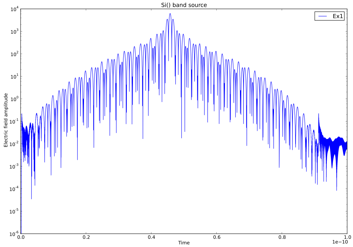
Si source: a) spectrum, b) time evolution
The Blackman-Nutall window guarrantees that the spectral wings drop to less than -50 dB after (2/t) frequency difference from the band edge.
In the case of unavailable GSL library, we may substitute Si() with the sinc function given as sin(t)/t. It does not give flat top in the band (its spectral amplitude is linearly sloped), but mostly it works, too.
 b)
b)
sinc source: a) spectrum, b) time evolution
Download the patches for meep 1.2.1 here:
After compilation of MEEP and Python-meep, the band-source can be directly substituted for the gaussian source:meep.band_src_time(model.srcFreq/c, model.srcWidth/c, model.simtime*c/1.1)Three parameters are required: the center frequency, the spectral width and the duration of the source (which determines how the band edges are sharp). For comparison, a gaussian source of similar function would look like this:
meep.gaussian_src_time(model.srcFreq/c, model.srcWidth/c)Unfortunately I did not check the scheme interface so far, but it should work as well. Write me in case of any problems.
Instabilities and other impertinencies
Although I often make mistakes and also MEEP itself has its bugs, time to time I encounter some issues with MEEP that arise from deeper background of FDTD simulation. I even would not call them numeric instabilites, because I think they may occur as a solution of the simulation setup, no matter how the math is precise. (But this does not mean that they couldn't and shouldn't be prevented.)
Checkerboard pattern on sharp dispersive interfaces
This happens when conductivity of metals is set too high. The simulation creates a pixelized field pattern on the surface of metal. It does not oscillate, but its amplitude grows exponentially and usually very fast (cca doubling each time step). I believe this is an issue discussed somewhere on the meep website, which is caused by the different location of E-field and H-field points (Yee grid). It seems that at the border, there occurs a "material" combined from the properties of air and metal (negative epsilon), which causes the field to diverge.
To avoid this issue, the metal conductivity has to be reduced. Fortunately, carefully setting even an unrealistic low value of conductivity may still allow the "metal" to behave as metal in the simulation. Take care of plasma frequency and skin depth.
This instability is directly related to the ratio of the sigma parameter and the Courant factor. Increasing the latter helps, too.
Sparkling on metallic corners (physical)
This is something related to localized surface plasmons; it is observed when the plasma frequency in metallic particles is similar to the source frequency. The sparkling, which looks very unphysically, is probably caused low resolution and by field enhancement on sharp corners.
So this is probably no error in MEEP at all. High-res simulations look much better.
I have ran series of simulations to understand this behaviour. If you are interested, write me an e-mail.
Resonator oscillations transverse to PML (solved in MEEP 1.2?)
When I set up a simulation of a nondispersive TiO2 sphere, in order to obtain its transmission and reflection spectra, I first observed that the calculation of S-parameters fails. In the time evolution of the reflected and transmitted fields was not only the original pulse (0-5 ps) and its ringdowns (5-100... ps), but also exponentially growing oscillations (from 300 ps). (See original mailinglist report.) The problematic script is here.

Time evolution of the reflected and tr. fields over 420 ps, showing beautiful oscillations
Originally I though that it is caused by wrong setting of material properties, but the problem persisted for simple nondispersive "epsilon=94" material. It needed a longer experimenting with MEEP to find the solution. It seems that a resonating structure has to be far away from any PML (perfectly matched layers), otherwise the near-field of the resonator couples somehow to the PML and starts oscillating.
 b)
b)  c)
c)  d)
d)  e)
e)  f)
f)  g)
g)  h)
h) 
a-h) Ex field in the Y-Z cut of the oscillations for different times in one half-period
The oscillations are mostly transverse and they do not occur if PMLs are added to all sides. It shall be noted that the energy buildup is quite strong, taking into account how fast the oscillations grow and that any transverse mode is attenuated by diffraction in the PMLs. Also interesting is that inside of the PMLs, the phase of the wave is shifted forwards by quarter of period.
The solution is to put the PML far from any resonator. Increasing the Z-size of the simulation volume from 200 um to 400 um prevents the oscillations for at least one 1000 picoseconds, which is enough for me. A fixed script can be found here.
I do not understand the mathematical background at all. Maybe, for some frequency, the resonator rotates the positive absorption of PML in the complex plane to a "negative absorption", i. e. amplification. If you solved this issue, I would be interested. (And on the other hand, if you replicated this behaviour in practice, you would solve the energy demands of mankind forever.)
EDIT 2013-01-10: I am convinced the problem is really in PML being able to amplify the evanescent waves in the near field of the oscillator. I tried to put a thin highly lossy medium into part of the PML volume. The propagating waves are attenuated enough by PML and do not reflect. The evanescent waves which freely pervade the PML are now attenuated in the lossy medium and the simulation is eventually stable.
There is one caveat: when the evanescent waves get attenuated, most of the resonances in the structure become damped. With the lossy medium or without it, one has to provide enough space around the structure if the narrow resonances are to be simulated properly! Otherwise it makes no sense to run a long simulation anyway.
I have also observed the case when losses and amplification nearly cancelled out and the resonances became narrow even in a small volume. However, generally it is much more practical to allocate a great simulation volume than to fine tune the losses in PML! It would be interesting if a evanescent-wave-friendly PML could be coded in MEEP in the future.
Further info: ab-initio.mit.edu/wiki/index.php/Perfectly_matched_layer
EDIT 2013-03-11: The meep 1.2 should fix this problem. I will have to experiment with this.
Divergence of frequency-domain solver
Using MEEP 1.2.1, I observed an instability complementary to the previous one: The frequency-domain solver diverged when the perfectly matched layers were too far from the simulated structure. Keeping the spacing in front of and behind the structure smaller than the real size of the structure mate the solver converge properly.
Harminv crashes with long simulation
Reported on Launchpad.
Harminv has rounding error with short simulation
Reported on Launchpad.
Related sofware
There are plenty of other electromagnetism programs, both commercial and free. I have found these freely available FDTD codes:
EMTL
EMTL is an open-source FDTD code developed by Kintech Lab.
From a brief reading of its documentation it seems that it has some interesting additional features such as modified Lorentz resonances, far-field calculation, tensor permittivity averaging for dispersive materials etc.
Comparing the features with MEEP, based on the website:
- + implemented precise tensor permittivity for dispersive media
- + implemented modified Lorentz term for dispersive media
- + several new clever algorithms
- - no python support?
- - smaller user base
B-CALM
B-CALM is another FDTD simulation which employs CUDA for superfast computing on the graphical card. It communicates via a HDF5 file. My compilation procedure.Comparing the features with MEEP, based on the website:
- + very fast GPU computation
- - using CUDA, depends on Nvidia cards
- - smaller user base
OpenEMS
OpenEMS is open-source FDTD code developed at the University of Duisburg
Comparing the features with MEEP, based on the website:
- + seems to be actively developed (as of 2012)
- + variable grid density
- + supplied with graphical interface CSXCAD (using VTK)
- + computation of far-field (radar cross-section etc.)
- . no Python support, but Octave is also OK
- - I did not make it compile on Ubuntu 12.10 (broken KDE dependency)
- - smaller user base?
http://openems.de/forum/viewtopic.php?f=4&t=92
CAMFR
It may be useful to complement MEEP with CAMFR. A straightforward procedure how to compile its latest version follows. (Tested on Ubuntu 12.10.)
#!/bin/bash
## Install the dependencies
sudo apt-get install libboost-python-dev scons libblitz-dev python-dev python-numpy liblapack-dev

## Get and unpack the sources
wget http://garr.dl.sourceforge.net/project/camfr/camfr/camfr-20070717/camfr-20070717.tgz
tar xzf camfr-20070717.tgz
cd camfr_20070717

## Change the options for compilation (removes the dependency on 'mkl' and 'g2c', but seems to work)
ln -s machine_cfg.py.gcc machine_cfg.py
sed -i -e 's|^flags = .*|flags = base_flags + "-O3 -march=native -g -funroll-loops "|g' machine_cfg.py
sed -i -e 's|^include_dirs = .*|include_dirs = ["/usr/include/python2.7", "/pymodules/python2.7/", \
	"/usr/lib/python2.7/dist-packages/"] |g' machine_cfg.py
sed -i -e 's|^libs = .*|libs = ["boost_python", "blitz", "lapack"]|g' machine_cfg.py

## Compile and install
sudo python setup.py install
The compilation takes no more than 5 minutes. Note this project has not been updated for few years and also some of its example files may have to be modified to work on 64-bit computers.
EMpy
Files
This section lists all the python programs that were referred to in the above text. All of them are free to use and redistribute, being licensed under the BSD license. They are often based on the work of many other MEEP users.
- meep_utils.py - many useful routines for simulations
- meep_materials.py - few classes defining Drude-Lorentz materials, may be easily extended
- run_sim.py - the main Python script that runs the MEEP as a library and exports the results
- view_meep.py - uses Mayavi2 to load the VTK output and show 3D visualisation of the structure and fields in one time snapshot
- README.txt - a license and description file